Пример машинного обучения
Ирэн Риверо (30 декабря 2022 г.)
Практический проект Прогнозирование риска рака шейки матки с помощью машинного обучения разделен на следующие задачи:
- Понять постановку проблемы и бизнес-кейс
- Импорт библиотек/наборов данных
- Выполните исследовательский анализ данных
- Выполнение визуализации данных
- Подготовьте данные перед обучением модели
- Обучение и оценка модели XG-Boost
Спасибо профессору Райану Ахмеду за то, что он сделал этот проект таким простым!
XGBoost
XGBoost или Extreme Gradient Boosting — это алгоритм, который выбирают многие специалисты по данным, и его можно использовать для задач регрессии и классификации. XGBoost — это алгоритм обучения под наблюдением, реализующий алгоритм деревьев с градиентным усилением.
Алгоритм работает путем объединения ансамбля прогнозов из нескольких слабых моделей. Он устойчив ко многим распределениям данных и отношениям и предлагает множество гиперпараметров для настройки производительности модели. XGBoost предлагает повышенную скорость и улучшенное использование памяти.
Усиление работает за счет обучения на предыдущих ошибках (ошибки в прогнозах модели) для создания лучших прогнозов на будущее. Повышение — это метод ансамблевого машинного обучения, который работает путем последовательного обучения слабых моделей.
Каждая модель пытается извлечь уроки из предыдущей слабой модели и стать лучше в прогнозировании. Алгоритмы повышения работают, строя модель из обучающих данных, затем вторая модель строится на основе ошибок (остатков) первой модели. Алгоритм повторяется до тех пор, пока не будет создано максимальное количество моделей или пока модель не будет давать хорошие прогнозы.
Понять формулировку проблемы
В этом практическом проекте мы создадим и обучим модель XGBoost для прогнозирования рака шейки маткиу 858 пациентов.
Набор данных был собран в «Университетской больнице Каракаса» в Каракасе, Венесуэла, и содержит демографическую информацию, привычки и исторические медицинские записи 858 пациентов.
Рак шейки матки убивает около 4 000 женщин в США и около 300 000 женщин во всем мире. Благодаря усилению медицинского скрининга смертность от рака шейки матки с 1955 по 1992 год снизилась на 74%.
Исследования показали, что высокая сексуальная активность и вирус папилломы человека (ВПЧ) являются одним из ключевых факторов, повышающих риск развития рака шейки матки.
Наличие гормонов в оральных контрацептивах, многодетность и курение повышают риск развития рака шейки матки, особенно у женщин, инфицированных ВПЧ. Кроме того, люди со слабой иммунной системой (ВИЧ/СПИД) имеют высокий риск заражения ВПЧ.

Импорт набора данных и библиотек
import pandas as pd
import numpy as np
import seaborn as sns
import matplotlib.pyplot as plt
import zipfile
!pip install jupyterthemes
!pip install plotly
import plotly.express as px
from jupyterthemes import jtplot
jtplot.style(theme = 'monokai', context = 'notebook', ticks = True, grid = False)
# setting the style of the notebook to be monokai theme
# this line of code is important to ensure that we are able to see the x and y axes clearly
# If you don't run this code line, you will notice that the xlabel and ylabel on any plot is black on black and it will be hard to see them.
# import the csv files using pandas
cancer_df = pd.read_csv('cervical_cancer.csv')
# (int) Age
# (int) Number of sexual partners
# (int) First sexual intercourse (age)
# (int) Num of pregnancies
# (bool) Smokes
# (bool) Smokes (years)
# (bool) Smokes (packs/year)
# (bool) Hormonal Contraceptives
# (int) Hormonal Contraceptives (years)
# (bool) IUD ("IUD" stands for "intrauterine device" and used for birth control
# (int) IUD (years)
# (bool) STDs (Sexually transmitted disease)
# (int) STDs (number)
# (bool) STDs:condylomatosis
# (bool) STDs:cervical condylomatosis
# (bool) STDs:vaginal condylomatosis
# (bool) STDs:vulvo-perineal condylomatosis
# (bool) STDs:syphilis
# (bool) STDs:pelvic inflammatory disease
# (bool) STDs:genital herpes
# (bool) STDs:molluscum contagiosum
# (bool) STDs:AIDS
# (bool) STDs:HIV
# (bool) STDs:Hepatitis B
# (bool) STDs:HPV
# (int) STDs: Number of diagnosis
# (int) STDs: Time since first diagnosis
# (int) STDs: Time since last diagnosis
# (bool) Dx:Cancer
# (bool) Dx:CIN
# (bool) Dx:HPV
# (bool) Dx
# (bool) Hinselmann: target variable - A colposcopy is a procedure in which doctors examine the cervix.
# (bool) Schiller: target variable - Schiller's Iodine test is used for cervical cancer diagnosis
# (bool) Cytology: target variable - Cytology is the exam of a single cell type used for cancer screening.
# (bool) Biopsy: target variable - Biopsy is performed by removing a piece of tissue and examine it under microscope,
# Biopsy is the main way doctors diagnose most types of cancer.
# Let's explore the dataframe
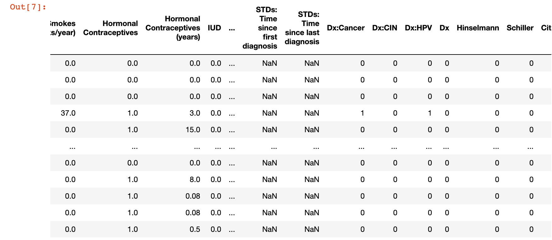
cancer_df

#Print the last 20 rows in the dataframe
cancer_df.tail(20)
#Print the first 20 rows in the dataframe
cancer_df.head(20)

Выполнение исследовательского анализа данных
# Get data frame info
cancer_df.info()

<class 'pandas.core.frame.DataFrame'>
RangeIndex: 858 entries, 0 to 857
Data columns (total 36 columns):
 #   Column                              Non-Null Count  Dtype
---  ------                              --------------  -----
 0   Age                                 858 non-null    int64
 1   Number of sexual partners           858 non-null    object
 2   First sexual intercourse            858 non-null    object
 3   Num of pregnancies                  858 non-null    object
 4   Smokes                              858 non-null    object
 5   Smokes (years)                      858 non-null    object
 6   Smokes (packs/year)                 858 non-null    object
 7   Hormonal Contraceptives             858 non-null    object
 8   Hormonal Contraceptives (years)     858 non-null    object
 9   IUD                                 858 non-null    object
 10  IUD (years)                         858 non-null    object
 11  STDs                                858 non-null    object
 12  STDs (number)                       858 non-null    object
 13  STDs:condylomatosis                 858 non-null    object
 14  STDs:cervical condylomatosis        858 non-null    object
 15  STDs:vaginal condylomatosis         858 non-null    object
 16  STDs:vulvo-perineal condylomatosis  858 non-null    object
 17  STDs:syphilis                       858 non-null    object
 18  STDs:pelvic inflammatory disease    858 non-null    object
 19  STDs:genital herpes                 858 non-null    object
 20  STDs:molluscum contagiosum          858 non-null    object
 21  STDs:AIDS                           858 non-null    object
 22  STDs:HIV                            858 non-null    object
 23  STDs:Hepatitis B                    858 non-null    object
 24  STDs:HPV                            858 non-null    object
 25  STDs: Number of diagnosis           858 non-null    int64
 26  STDs: Time since first diagnosis    858 non-null    object
 27  STDs: Time since last diagnosis     858 non-null    object
 28  Dx:Cancer                           858 non-null    int64
 29  Dx:CIN                              858 non-null    int64
 30  Dx:HPV                              858 non-null    int64
 31  Dx                                  858 non-null    int64
 32  Hinselmann                          858 non-null    int64
 33  Schiller                            858 non-null    int64
 34  Citology                            858 non-null    int64
 35  Biopsy                              858 non-null    int64
dtypes: int64(10), object(26)
memory usage: 241.4+ KB
# Get the statistics of the data frame
cancer_df.describe()

# Notice many question marks indicating missing values
cancer_df

# Let's replace '?' with NaN
cancer_df = cancer_df.replace('?', np.nan)
cancer_df
cancer_df.isnull()

# Plot heatmap
plt.figure(figsize = (20, 20))
sns.heatmap(cancer_df.isnull())

# Get data frame info
cancer_df.info()

<class 'pandas.core.frame.DataFrame'>
RangeIndex: 858 entries, 0 to 857
Data columns (total 36 columns):
 #   Column                              Non-Null Count  Dtype
---  ------                              --------------  -----
 0   Age                                 858 non-null    int64
 1   Number of sexual partners           832 non-null    object
 2   First sexual intercourse            851 non-null    object
 3   Num of pregnancies                  802 non-null    object
 4   Smokes                              845 non-null    object
 5   Smokes (years)                      845 non-null    object
 6   Smokes (packs/year)                 845 non-null    object
 7   Hormonal Contraceptives             750 non-null    object
 8   Hormonal Contraceptives (years)     750 non-null    object
 9   IUD                                 741 non-null    object
 10  IUD (years)                         741 non-null    object
 11  STDs                                753 non-null    object
 12  STDs (number)                       753 non-null    object
 13  STDs:condylomatosis                 753 non-null    object
 14  STDs:cervical condylomatosis        753 non-null    object
 15  STDs:vaginal condylomatosis         753 non-null    object
 16  STDs:vulvo-perineal condylomatosis  753 non-null    object
 17  STDs:syphilis                       753 non-null    object
 18  STDs:pelvic inflammatory disease    753 non-null    object
 19  STDs:genital herpes                 753 non-null    object
 20  STDs:molluscum contagiosum          753 non-null    object
 21  STDs:AIDS                           753 non-null    object
 22  STDs:HIV                            753 non-null    object
 23  STDs:Hepatitis B                    753 non-null    object
 24  STDs:HPV                            753 non-null    object
 25  STDs: Number of diagnosis           858 non-null    int64
 26  STDs: Time since first diagnosis    71 non-null     object
 27  STDs: Time since last diagnosis     71 non-null     object
 28  Dx:Cancer                           858 non-null    int64
 29  Dx:CIN                              858 non-null    int64
 30  Dx:HPV                              858 non-null    int64
 31  Dx                                  858 non-null    int64
 32  Hinselmann                          858 non-null    int64
 33  Schiller                            858 non-null    int64
 34  Citology                            858 non-null    int64
 35  Biopsy                              858 non-null    int64
dtypes: int64(10), object(26)
memory usage: 241.4+ KB
# Since STDs: Time since first diagnosis  and STDs: Time since last diagnosis have more than 80% missing values
# we can drop them
cancer_df = cancer_df.drop(columns = ['STDs: Time since first diagnosis', 'STDs: Time since last diagnosis'])

cancer_df

# Since most of the column types are object, we are not able to get the statistics of the dataframe.
# Convert them to numeric type

cancer_df = cancer_df.apply(pd.to_numeric)
cancer_df.info()

<class 'pandas.core.frame.DataFrame'>
RangeIndex: 858 entries, 0 to 857
Data columns (total 34 columns):
 #   Column                              Non-Null Count  Dtype
---  ------                              --------------  -----
 0   Age                                 858 non-null    int64
 1   Number of sexual partners           832 non-null    float64
 2   First sexual intercourse            851 non-null    float64
 3   Num of pregnancies                  802 non-null    float64
 4   Smokes                              845 non-null    float64
 5   Smokes (years)                      845 non-null    float64
 6   Smokes (packs/year)                 845 non-null    float64
 7   Hormonal Contraceptives             750 non-null    float64
 8   Hormonal Contraceptives (years)     750 non-null    float64
 9   IUD                                 741 non-null    float64
 10  IUD (years)                         741 non-null    float64
 11  STDs                                753 non-null    float64
 12  STDs (number)                       753 non-null    float64
 13  STDs:condylomatosis                 753 non-null    float64
 14  STDs:cervical condylomatosis        753 non-null    float64
 15  STDs:vaginal condylomatosis         753 non-null    float64
 16  STDs:vulvo-perineal condylomatosis  753 non-null    float64
 17  STDs:syphilis                       753 non-null    float64
 18  STDs:pelvic inflammatory disease    753 non-null    float64
 19  STDs:genital herpes                 753 non-null    float64
 20  STDs:molluscum contagiosum          753 non-null    float64
 21  STDs:AIDS                           753 non-null    float64
 22  STDs:HIV                            753 non-null    float64
 23  STDs:Hepatitis B                    753 non-null    float64
 24  STDs:HPV                            753 non-null    float64
 25  STDs: Number of diagnosis           858 non-null    int64
 26  Dx:Cancer                           858 non-null    int64
 27  Dx:CIN                              858 non-null    int64
 28  Dx:HPV                              858 non-null    int64
 29  Dx                                  858 non-null    int64
 30  Hinselmann                          858 non-null    int64
 31  Schiller                            858 non-null    int64
 32  Citology                            858 non-null    int64
 33  Biopsy                              858 non-null    int64
dtypes: float64(24), int64(10)
memory usage: 228.0 KB
# Get the statistics of the dataframe
cancer_df.describe()

cancer_df.mean()

Age                                   26.820513
Number of sexual partners              2.527644
First sexual intercourse              16.995300
Num of pregnancies                     2.275561
Smokes                                 0.145562
Smokes (years)                         1.219721
Smokes (packs/year)                    0.453144
Hormonal Contraceptives                0.641333
Hormonal Contraceptives (years)        2.256419
IUD                                    0.112011
IUD (years)                            0.514804
STDs                                   0.104914
STDs (number)                          0.176627
STDs:condylomatosis                    0.058433
STDs:cervical condylomatosis           0.000000
STDs:vaginal condylomatosis            0.005312
STDs:vulvo-perineal condylomatosis     0.057105
STDs:syphilis                          0.023904
STDs:pelvic inflammatory disease       0.001328
STDs:genital herpes                    0.001328
STDs:molluscum contagiosum             0.001328
STDs:AIDS                              0.000000
STDs:HIV                               0.023904
STDs:Hepatitis B                       0.001328
STDs:HPV                               0.002656
STDs: Number of diagnosis              0.087413
Dx:Cancer                              0.020979
Dx:CIN                                 0.010490
Dx:HPV                                 0.020979
Dx                                     0.027972
Hinselmann                             0.040793
Schiller                               0.086247
Citology                               0.051282
Biopsy                                 0.064103
dtype: float64
# Replace null values with mean
cancer_df = cancer_df.fillna(cancer_df.mean())

cancer_df

# Nan heatmap
plt.figure(figsize = (20,20))
sns.heatmap(cancer_df.isnull(), yticklabels = False)

#What is the age range of people involved in this study?
#What are the biopsy results for the oldest person in this study?

cancer_df['Age'].min()
13

cancer_df['Age'].max()
84

cancer_df[cancer_df['Age'] == 84]

Выполнить визуализацию данных
# Get the correlation matrix
corr_matrix=cancer_df.corr()

corr_matrix

# Plot the correlation matrix
plt.figure(figsize = (30, 30))
sns.heatmap (corr_matrix, annot =True)
plt.show()

fig = px.bar(cancer_df, x="Age", y="Biopsy", orientation='h', color = 'Age', labels = dict(Age = 'Total Instances'))
fig.show()

#Plot the histogram for the entire DataFrame
cancer_df.hist(bins=10, figsize = (30, 30), color= 'b')

Подготовьте данные перед обучением
target_df = cancer_df ['Biopsy']
input_df = cancer_df.drop(columns = ['Biopsy'])

target_df.shape
(858,)

input_df.shape
(858, 33)

target_df
0      0
1      0
2      0
3      0
4      0
      ..
853    0
854    0
855    0
856    0
857    0
Name: Biopsy, Length: 858, dtype: int64

X = np.array(input_df).astype('float32')
y = np.array(target_df).astype('float32')

# reshaping the array from (421570,) to (421570, 1)
# y = y.reshape(-1,1)
y.shape
(858,)

# scaling the data before feeding the model
from sklearn.preprocessing import StandardScaler, MinMaxScaler
scaler = StandardScaler()
X = scaler.fit_transform(X)

X

array([[-1.0385634e+00,  8.9706147e-01, -7.1509570e-01, ...,
        -2.0622157e-01, -3.0722591e-01, -2.3249528e-01],
       [-1.3917956e+00, -9.3074709e-01, -1.0734857e+00, ...,
        -2.0622157e-01, -3.0722591e-01, -2.3249528e-01],
       [ 8.4534228e-01, -9.3074709e-01,  2.2945171e-07, ...,
        -2.0622157e-01, -3.0722591e-01, -2.3249528e-01],
       ...,
       [-2.1435463e-01, -3.2147753e-01,  1.6845580e-03, ...,
        -2.0622157e-01, -3.0722591e-01,  4.3011627e+00],
       [ 7.2759819e-01, -3.2147753e-01,  2.5104153e+00, ...,
        -2.0622157e-01, -3.0722591e-01, -2.3249528e-01],
       [ 2.5662178e-01, -3.2147753e-01,  1.0768549e+00, ...,
        -2.0622157e-01, -3.0722591e-01, -2.3249528e-01]], dtype=float32)


# scaler = StandardScaler()
# X_train = scaler.fit_transform(X_train)
# X_test = scaler.transform(X_test)
# X_val = scaler.transform(X_val)

# spliting the data in to test and train sets
from sklearn.model_selection import train_test_split

X_train, X_test, y_train, y_test = train_test_split(X, y, test_size = 0.2)
X_test, X_val, y_test, y_val = train_test_split(X_test, y_test, test_size = 0.5)

#Split the data such that the testing data is quarter the size of the training data
X_train, X_test, y_train, y_test = train_test_split(X, y, test_size = 0.25)
Обучение и оценка классификатора XGBoost
!pip install xgboost

# Train an XGBoost classifier model
import xgboost as xgb

model = xgb.XGBClassifier(learning_rate = 0.1, max_depth = 5, n_estimators = 10)

model.fit(X_train, y_train)

result_train = model.score(X_train, y_train)
print("Accuracy : {}".format(result_train))

Accuracy : 0.9860031104199067

# predict the score of the trained model using the testing dataset
result_test = model.score(X_test, y_test)
print("Accuracy : {}".format(result_test))

Accuracy : 0.9441860465116279

# make predictions on the test data
y_predict = model.predict(X_test)

from sklearn.metrics import confusion_matrix, classification_report
print(classification_report(y_test, y_predict))

              precision    recall  f1-score   support

         0.0       0.95      0.99      0.97       194
         1.0       0.85      0.52      0.65        21

    accuracy                           0.94       215
   macro avg       0.90      0.76      0.81       215
weighted avg       0.94      0.94      0.94       215
cm = confusion_matrix(y_predict, y_test)
sns.heatmap(cm, annot = True)

plt.figure(figsize=(10, 10))
cm = confusion_matrix(y_predict, y_test)
sns.heatmap(cm, annot = True,fmt = '.2f')
plt.ylabel('Predicted class')
plt.xlabel('Actual class')

#Retrain the model with 10x and 100x the number of estimators and tree depth
#Plot the confusion matrix
#Comment on the performance of the mode

model = xgb.XGBClassifier(learning_rate = 0.1, max_depth = 50, n_estimators = 100)

model.fit(X_train, y_train)

result_train = model.score(X_train, y_train)
print("Accuracy : {}".format(result_train))

Accuracy : 0.9956268221574344

# predict the score of the trained model using the testing dataset
result = model.score(X_test, y_test)
print("Accuracy : {}".format(result))

Accuracy : 0.9651162790697675

# make predictions on the test data
y_predict = model.predict(X_test)

from sklearn.metrics import confusion_matrix, classification_report
print(classification_report(y_test, y_predict))

              precision    recall  f1-score   support

         0.0       0.99      0.97      0.98        80
         1.0       0.71      0.83      0.77         6

    accuracy                           0.97        86
   macro avg       0.85      0.90      0.88        86
weighted avg       0.97      0.97      0.97        86
plt.figure(figsize=(10, 10))
cm = confusion_matrix(y_predict, y_test)
sns.heatmap(cm, annot = True,fmt = '.2f')
plt.ylabel('Predicted class')
plt.xlabel('Actual class')

Попытка получить лучшую поддержку
X_train, X_test, y_train, y_test = train_test_split(X, y, test_size = 0.25)

model = xgb.XGBClassifier(learning_rate = 0.1, max_depth = 50, n_estimators = 100)

model.fit(X_train, y_train)
XGBClassifier(max_depth=50)

result_train = model.score(X_train, y_train)
print("Accuracy : {}".format(result_train))
Accuracy : 1.0

result = model.score(X_test, y_test)
print("Accuracy : {}".format(result))
Accuracy : 0.9627906976744186

y_predict = model.predict(X_test)

from sklearn.metrics import confusion_matrix, classification_report
print(classification_report(y_test, y_predict))

              precision    recall  f1-score   support

         0.0       0.98      0.98      0.98       205
         1.0       0.60      0.60      0.60        10

    accuracy                           0.96       215
   macro avg       0.79      0.79      0.79       215
weighted avg       0.96      0.96      0.96       215
plt.figure(figsize=(10, 10))
cm = confusion_matrix(y_predict, y_test)
sns.heatmap(cm, annot = True,fmt = '.2f')
plt.ylabel('Predicted class')
plt.xlabel('Actual class')
